Lesson One Big O Complexity
This article series is written firstly for my own understanding and I write it to become better at Algorithms but also at writing on technical topics. Follow along and hopefully learn something.
What is this Big O Complexity that every fancy Software engineer is talking about. Just kidding it is mostly the algo champions or engineers wanting to land a job at the Big Dog companies that is talking about them.
My personal opinion is that Knowledge is always great and being good at Algorithms can come in hand but not a day to day crucial skill for most engineers (If we talk about all the stuff with different sorting algorithms etc).
So what is the Fuzz all about?
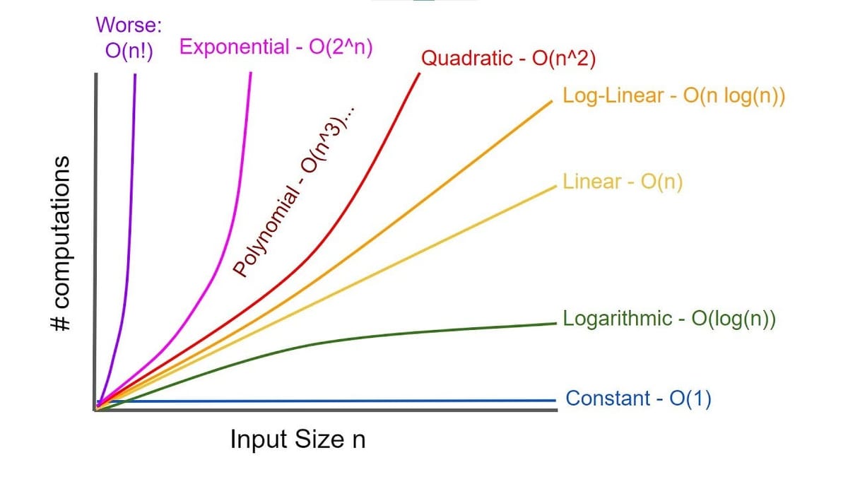
In Computer Science Big O notation is a term used to classify algorithms to how their run time or space requirements grow as the input size grows.
Okey that is great but what does it actually mean? What is O and what is N?
Big O notation is used to calculate the time our algorithm takes to run as the input grows. O is the whole operation and n is the input here.
I am a node developer by heart so all the code will be written in node here on forward. Sorry all python suckers.
O(n) Linear
O(n) means the time it will take the algorithm to execute grows linearly with the size of the input. In other words. Whenever input size changes the time it will take to execute will also correlate to the input size.
If the array has n elements the algorithm will perform a single operation for each element resulting in n operations.
Here we have a node example demonstrating this.
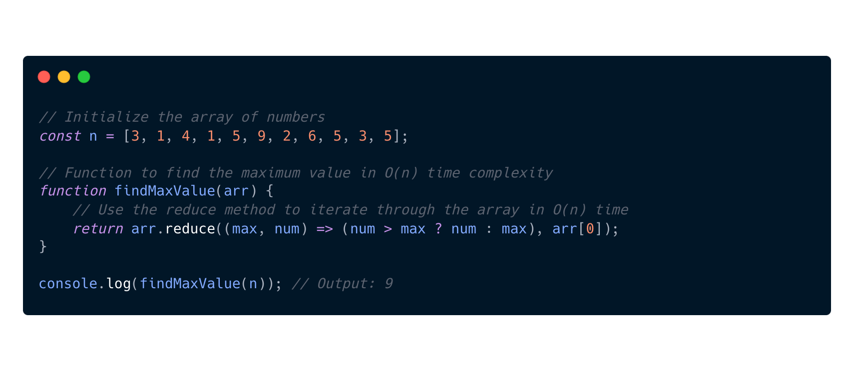
So why is this example O(n)?
- Reduce iterates from the first element to the last element of the array and visiting each element exactly one time
- Constant work per element. Comparisons, conditional statements and assignments are constant-time operations of O(1).
- And since these operations are performed for each element in the array when looping over the total work here is proportional to the number of elements in the array.
- We are just looping over each element one time and don't need to visit the same element multiple times and we don't have nested loops or recursive calls.
O(1) Constant
If we look at the previous example we see that I wrote about the O(1) Constant complexity. This is a complexity that doesn't depend on the size of the input. It will perform a constant number of operations and not tied to the input size.
Here we have two node example demonstrating this.

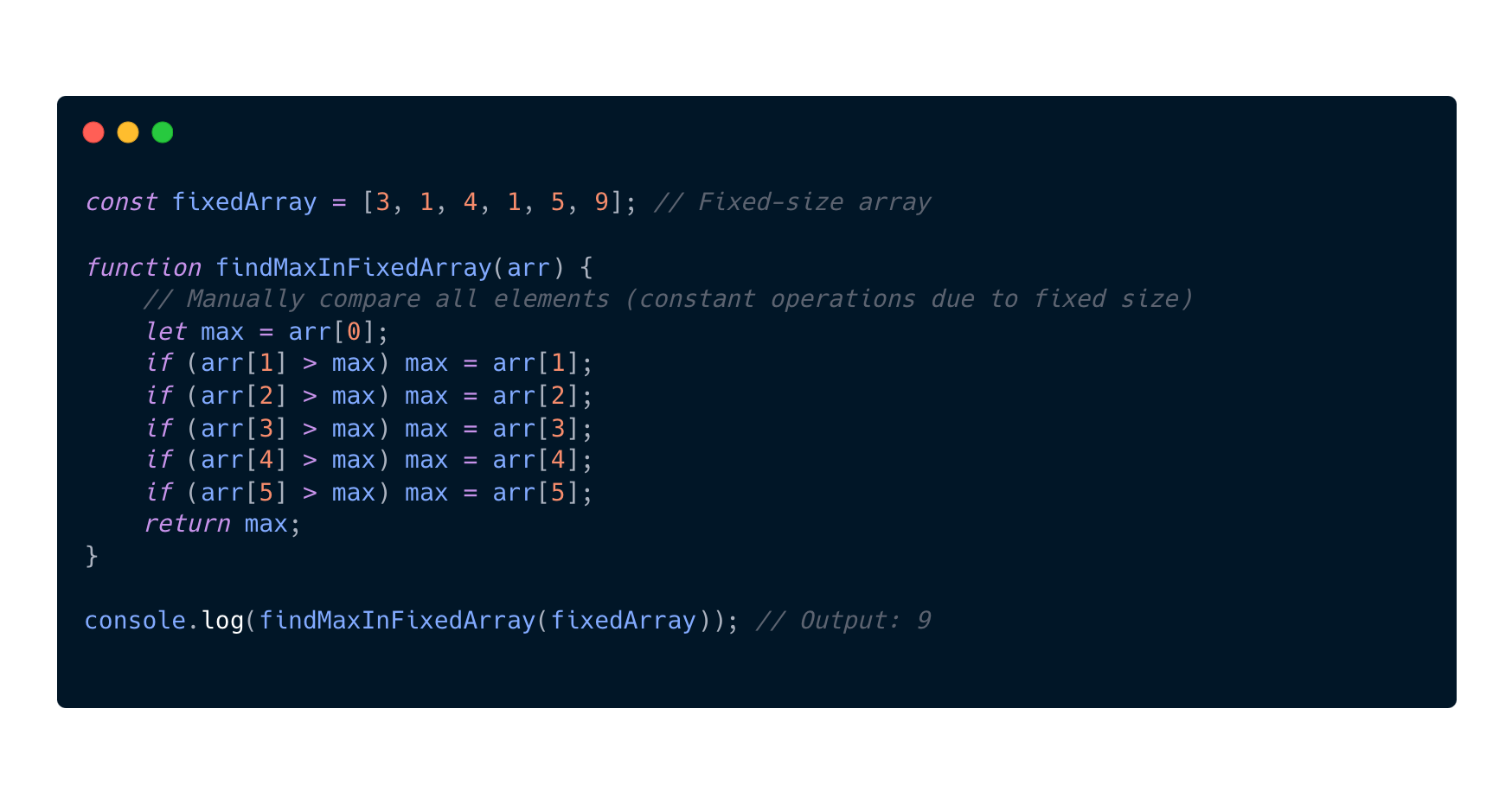
So why are these examples O(1)?
I provide two examples to give you a perspective on that these two types of functions are actually the same size of O(1) complexity. But how is that possible?
If the size of the array is constant as in this example and will not change, the algorithm's complexity becomes O(1). And in the first example we see that the getMaxValue function has a constant value and with constants or comparisons we get O(1) complexity.
O(n^2) Quadratic
Okey things are getting more and more advanced now and is also affecting the complexity more and more. Here we are talking about Quadratic complexity. In simple terms this is when dealing with nested loops that iterates over the same dataset in the outer and inner loop.

So why are this example O(n^2)?
If we look at the findMaxPairSum function we can identify a few things.
- Outer loop: Runs once for each element in the array(n times)
- For every iteration of the outer loop, the inner loop will run n times. The inner loop executes n times for each of the n iterations of the outer loop.
- Then we will actually start to look into how many total iterations this will take. And the formula for that will then be n x n = n^2
- And to sum that up with the input growth is getting higher we can see that the iterations is growing quadratically.
- n = 5, iterations = 5^2 = 25
- n = 100, iterations = 100^2 = 10 000
O(n^3) Polynomial
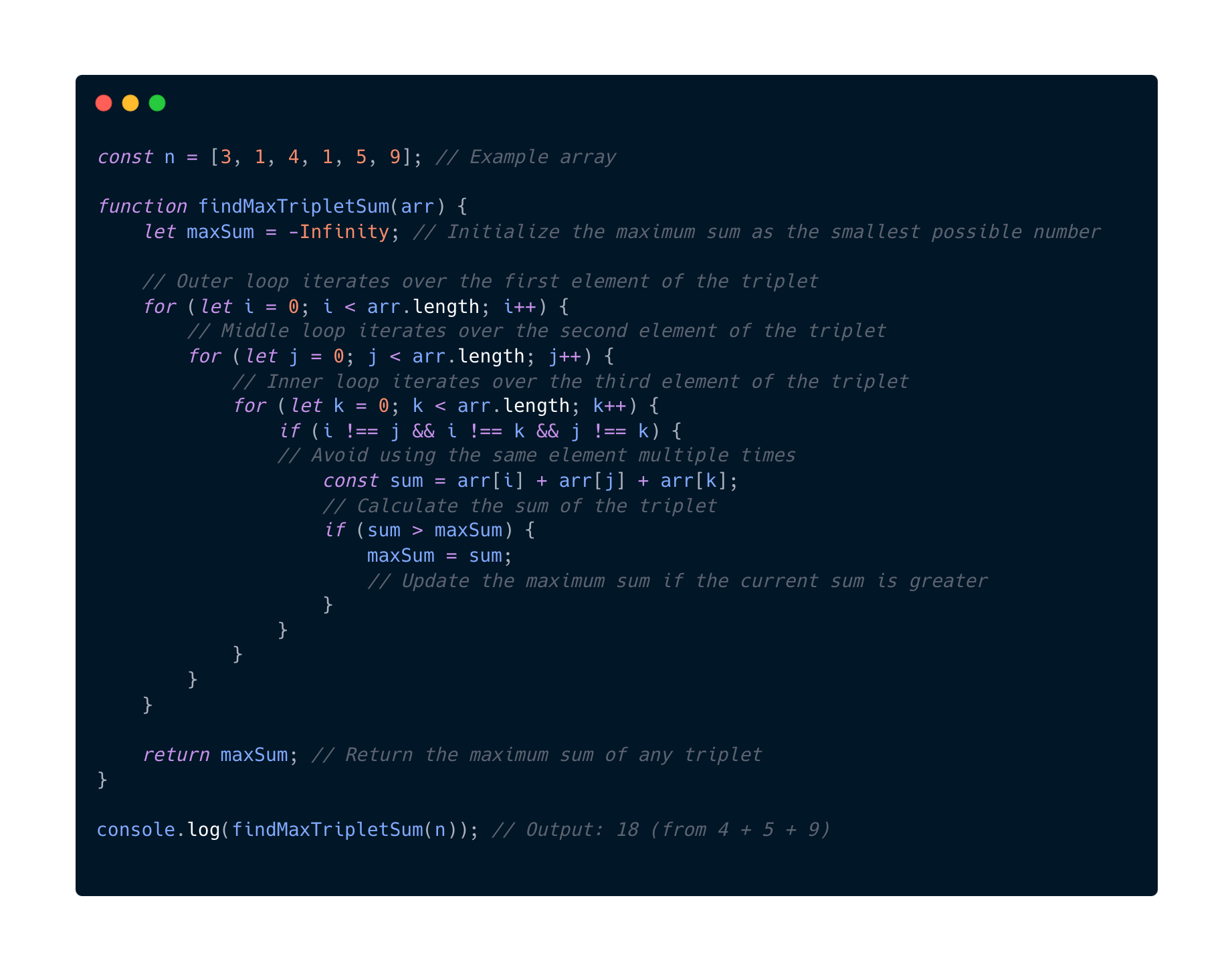
Now we are adding even more complexity to handle. Here we have a example of operations on the same dataset in three loops at the same time.
That means our complexity will look like n x n x n = n^3
This is the same example like we did see in the O(n^2) complexity space.
- n = 5, iterations = 5^3 = 125
- n = 100, iterations = 100^3 = 1 000 000
O(2^n) Exponential
I guess you all have heard about the fibonacci sequence. A famous interview question for technical interviews. At least here in Sweden. Here is a naive implementation to demonstrate the complexity for O(2^n).
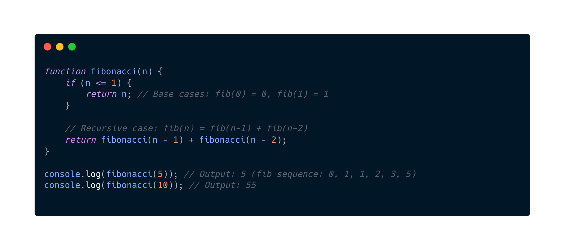

For this naive implementation of the fibonacci we can already see here in this example that the function fibonacci calls itself twice. And to highlight what the result will end up here is that it will result in a binary tree of recursive calls, where each level doubles the number of calls from the previous level.
So that means at each level i there are 2^i calls
O(n!) Factorial
Now we are in some deep as complexity and no go zone 🗡️
O(n!) algorithms are common in Permutations and Combinatorics Problems and in Backtracking Algorithms like finding all possible solutions to a problem. So lets check that out.
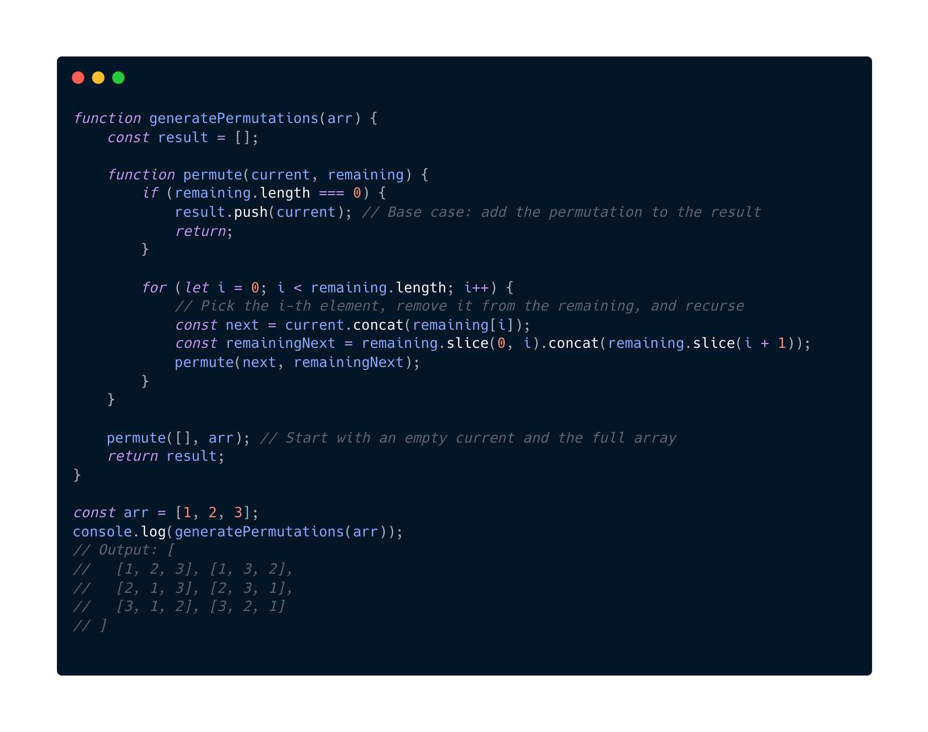
Lets see for the array of size n:
- Lets look at the first level. There are n choices
- At our second level here there are n - 1 choices
- Our third level there are n n - 2 choices, and so on.
So with that said the total work of permutations generated is n!
O(log(n)) Logarithmic
Now we are getting to the good stuff. This O complexity algorithm reduces the problem size by a factor. It is usually by half with each iteration or recursive step. It is commonly used in problems when solving binary search, divide-and-conquer strategies or tree traversals.
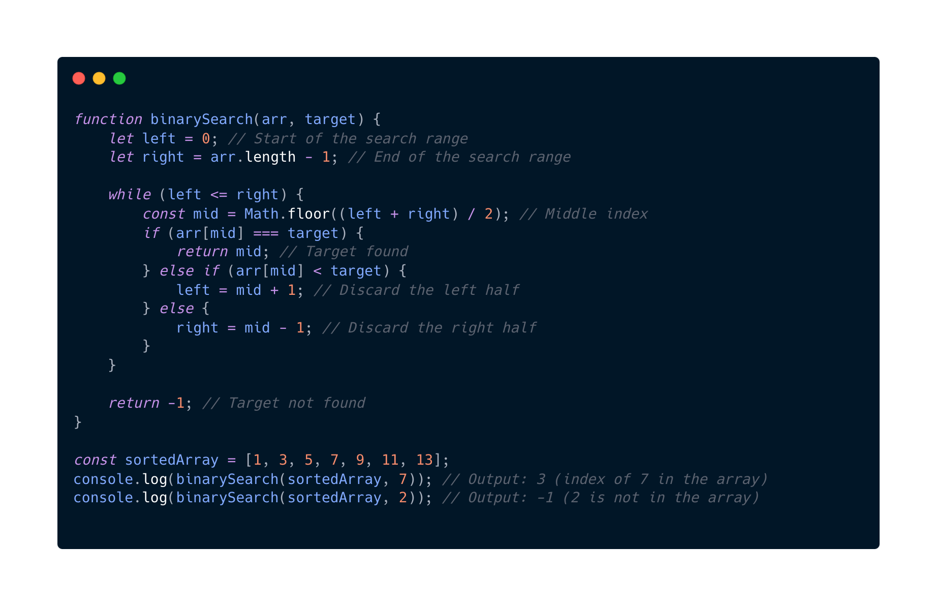
Some things to keep in mind here is that when using this algorithm the input need to be structured in a way that allows dividing the problem size efficiently.
- Binary search for example works only on sorted arrays.
- Divide-and-conquer requires the problem to be divisible.
- If we have data that is not structured or sorted properly the complexity might be O(n) or worse
O(n log(n)) Log Linear
This algorithm combines two algorithms. Linear and Logarithmic complexities. This is what we mostly see in Merge sort, Quick Sort or Heap Sort.
The O(log(n)) factor usually comes from a recursive divide-and-conquer strategy, while the O(n) comes from merging or partitioning.
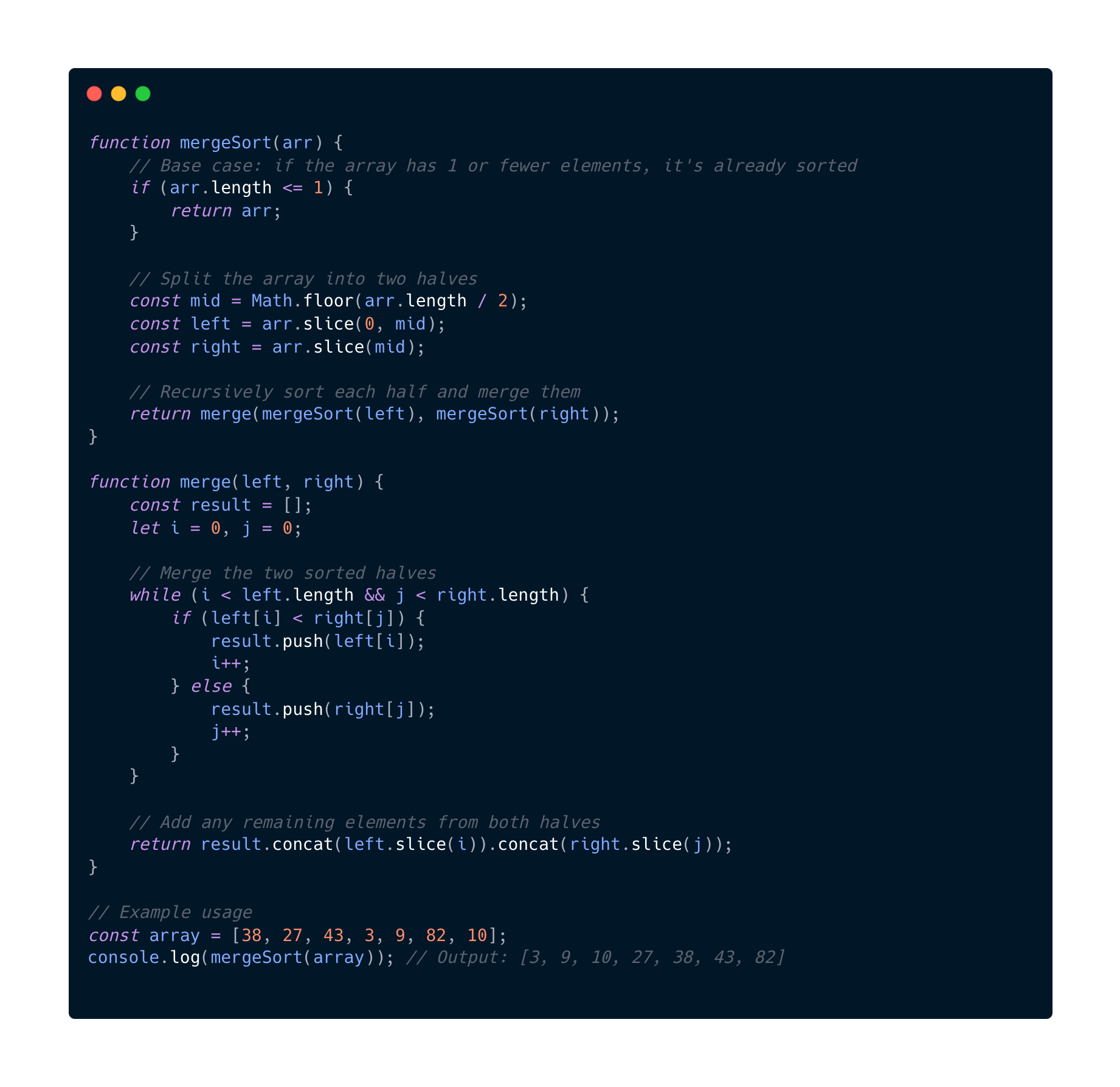
Why is this O(n log(n))?
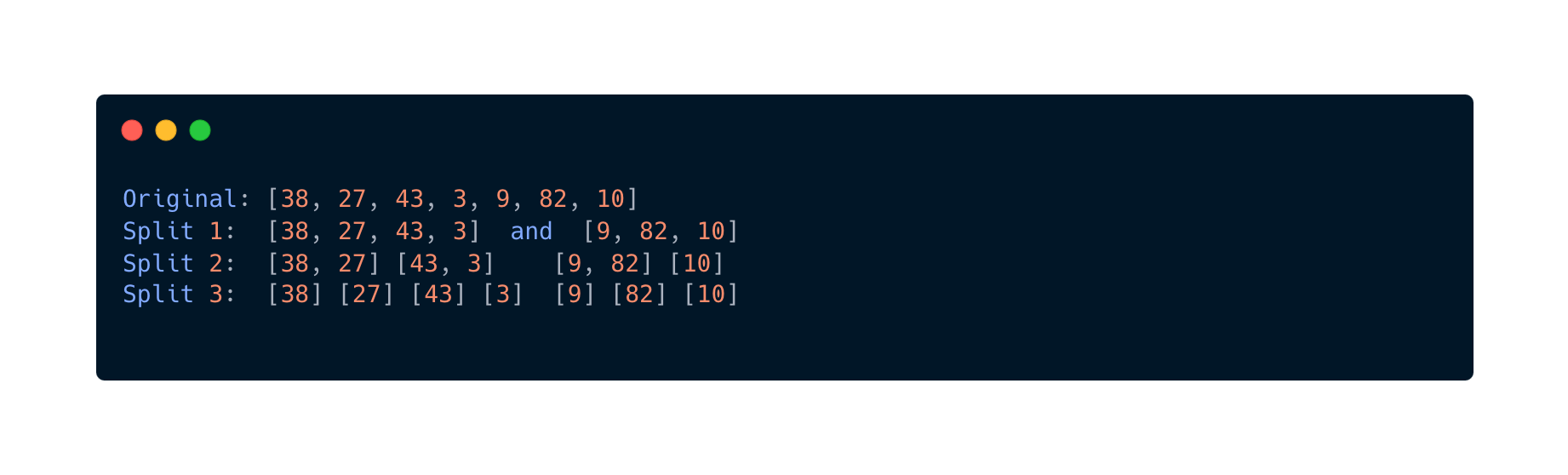
- Splitting the array: O(log(n))
- Merging the arrays O(n)
- Total work is therefore O(n) x O(log(n)) = O(n log(n))
When running this code this is how the splitting and merging works

And that's a wrap. This was really helpful for me to see some good examples of the different complexities. Next up I will deep dive and solve one problems in different time complexities to actually see some differences.
Stay tuned!